This guide shows you how to replace an MS Query connection with Power Query, Microsoft's newer tool for pulling data from a database into Excel. You build the new table first, check it matches, and only then remove the old one. Your sheet, formulas and reports keep working.
Term | Meaning |
MS Query | The old tool that fetches database data into a sheet |
Power Query | The newer tool that does the same job (Data > Get Data) |
Connection | The saved link between the workbook and the database |
Refresh | Fetching the latest data from the database |
On this page
Before You Start
- Save a copy of the workbook and work in the copy.
- Use Excel for Windows (Microsoft 365, or Excel 2016 or later).
- Have your database login ready, and check the old workbook refreshes on your computer today.
- If the file name ends in .xlsm, it contains macros. Ask IT to check them at the end.
- Do one table at a time.
- All Power Query users must be created as SQL users and assigned the appropriate SQL Roles by Tes Support.
- Do one table at a time.
Two Methods
Method #1 (Create query)
✅ Find the MS Query table
✅ See what the old query does
✅ Check what uses the table
✅ Connect with Power Query
✅ Match the old table
✅ Check the data matches
✅ Swap the new table in
Method #2 (Reuse an Existing MS Query SQL Statement - Advanced)
✅ Use headings to make text bigger
✅ See what the old query does
✅ Check what uses the table
✅ Change text colours manually
Method #1 Steps
Step 1: Find the MS Query table
- Go to Data > Queries & Connections and click the Connections tab in the panel on the right.
- Right-click the connection and choose Properties. The Used In tab shows the sheet and cells it fills.
- On the Definition tab, note the name after DSN= in the connection string. On the Usage tab, note which refresh options are ticked. Click Cancel.
- Click inside the table on the sheet and note its name from Table Design > Table Name.
Step 2: See what the old query does
- Right-click inside the old table and choose Table > Edit Query. The MS Query window opens.
- Note down what you see: the database table(s) at the top, the columns shown, any filters in the Criteria area (turn it on with View > Criteria if it's hidden), and how the rows are sorted.
- Close it with File > Cancel and Return to Microsoft Excel, so nothing changes.
If MS Query says the query can't be shown graphically, it was written by hand. Ask IT to help with that one.
Step 3: Check what uses the table
Go to Home > Find & Select > Find, click Options, set Within to Workbook and Look in to Formulas, type the table name and click Find All. Then click inside each PivotTable and check PivotTable Analyze > Change Data Source. Note anything that uses the table.
Step 4: Connect with Power Query
- Go to Data > Get Data > From Database > From SQL Server Database.
- Pick the DSN name you noted in Step 1 and click OK.
- Sign in to the database if asked.
- In the Navigator window, open the list and tick the same database table you noted in Step 2.
- Click Transform Data. The Power Query Editor opens.
Note! Some early Excel 2016 versions display Power Query as New Query rather than Get Data. Look under:
Data → New Query → From File / From Database
Step 5: Match the old table
Use your notes from Step 2. In the Power Query Editor:
- Columns: click Home > Choose Columns and tick only the columns the old query used.
- Filters: click the arrow on a column heading and set the same filter as the old query's criteria.
- Sort: use the same arrow to sort the same way.
- Headings and order: double-click a heading to rename it so it matches the old table exactly. Drag columns into the same order.
- Types: click the icon on each heading. Set dates to Date, and IDs that start with zero to Text.
If the old query used more than one database table, ask IT to help combine them.
When it looks right, click Home > Close & Load To, choose Table and New worksheet, and click OK.
Step 6: Check the data matches
Click Data > Refresh. Select a whole column in the old table and look at the bar at the bottom of the Excel window, which shows Count (and Sum for numbers). Select the same column in the new table. The numbers should match. Then compare a few rows by eye.
If something is different, right-click the query in Queries & Connections, choose Edit, fix it, and check again.
Step 7: Swap the new table in
- Remove the old connection. In Queries & Connections > Connections, right-click the MS Query connection and choose Delete. The old table keeps its data but no longer refreshes.
- Move the table name across (only if Step 3 found formulas using it). In Table Design > Table Name, rename the old table to OLD_Table, then give the new table the original name. Go to Home > Find & Select > Replace, click Options, set Within to Workbook and Look in to Formulas, and replace OLD_Table with the original name.
- Clear the old table. Select all of it, including headings, and choose Home > Clear > Clear All. Don't delete rows or columns, as that can break formulas.
- Move the new table in. Select the whole new table, right-click and choose Cut (not Copy). Right-click the old table's top-left cell and choose Paste.
- Right-click the table and choose Refresh to confirm it works. Delete the empty extra sheet.
Step 8: Finish up
- In Queries & Connections > Queries, right-click the query, choose Properties, and tick the same refresh options you noted in Step 1.
- Point any PivotTables at the table name (PivotTable Analyze > Change Data Source) and refresh them.
- Save, close, reopen and click Data > Refresh to confirm everything works.
Other users will be asked to sign in to the database the first time they refresh.
If something goes wrong
Problem | Fix |
Login keeps failing | Data > Get Data > Data Source Settings, select the database, Clear Permissions, then refresh and sign in again. |
Formula.Firewall or privacy level error | In Data Source Settings, click Edit Permissions and set both sources to the same privacy level (usually Organizational). |
Can't paste the new table | Some of the old table is still there. Clear the whole area again with Clear All. |
Formulas show #REF! | Close without saving, reopen your copy and redo Step 7 using Clear All, not Delete. |
Method #2 Steps
Step 1:
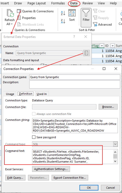
Open the existing MS Query report and select View > SQL.
Step 2:
Copy the SQL statement used by the report.
IMPORTANT: Remove all database references before using the SQL in Power Query. Example: SynergyOne.dbo.STUDENT becomes dbo.STUDENT.
Step 3:
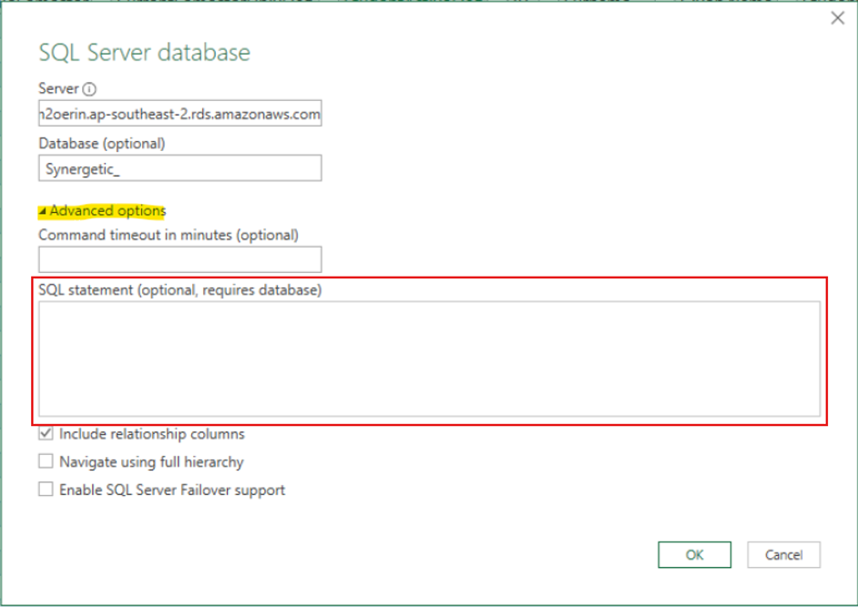
Create a SQL Server Database connection using Data > Get Data > From Database > From SQL Server Database.
Step 4:
Paste the modified SQL statement into Advanced Options.
Step 5:
Review the results and Close & Load the query.
Troubleshooting
Problem | Resolution |
Login keeps failing | Clear permissions and reconnect. |
Privacy errors | Set all sources to the same privacy level. |
SQL connection errors | Verify SQL Roles with Tes Global Support. |
SQL query fails | Remove database and schema names from table references. |
Additional Resources
Was this article helpful?
That’s Great!
Thank you for your feedback
Sorry! We couldn't be helpful
Thank you for your feedback
Feedback sent
We appreciate your effort and will try to fix the article